This paper is from machine learning coursework completed in a group of 5 during the Fall 2023 semester, in which we explored the benefits of neural network knowledge transfer.
Abstract
This report presents an analysis of transfer learning in machine learning, with a focus on medical image classification. The study begins by training a ResNet18 model on the Colorectal Cancer Classification (CCC) dataset. This model is then used to extract features from two other datasets: Prostate Cancer Classification (PCC) and Animal Faces Classification (AFC), to assess the effectiveness of transfer learning across different domains. The extracted features for the PCC dataset are analyzed using Random Forest and K-Nearest Neighbors (KNN) classifiers to evaluate their classification performance. The results are quantified using metrics such as precision, recall, and F1-score, and visually represented through t-SNE plots. The resulting f1-score of the RF and KNN classifiers on the PCC dataset are 0.90 and 0.88, demonstrating an effective knowledge transfer. The findings highlight both the strengths and limitations of transfer learning, offering valuable insights into its application in scenarios with limited labeled data and varying domain specificity.
Introduction
Knowledge transfer is a concept in the Machine Learning field where the knowledge of an already trained machine learning model is applied to a different problem, exploiting what has already been learned by one model to improve performance. Transfer learning addresses the lack of available labeled data by allowing a model to learn from related tasks and apply this knowledge to improve performance in a target task. Transfer learning has two main approaches, developing a model explicitly designed for transfer learning or utilizing a pre-trained model. The latter involves using existing models trained on large datasets for generic tasks, making them suitable for general usage rather than specific tasks (TL2). The preferred approach is situational and depends on task specificity, and available resources (TL3). Transfer learning is most successful when the source model is complex and shares domain and task similarity (TL1). Thus, challenges in transfer learning arises when the source model and target model domains differ as they are likely to have different features and weights attached to said features, and so could result in suboptimal performance. The same can be said for task dissimilarities between models. The expected results of the effective use of transfer learning are improved performance on a target task after fewer epochs than if the model were developed from scratch. When knowledge transfer is not used effectively it can lead to suboptimal performance, inefficient use of computational resources, limited model generalization, and increased training time (TL1). To acquire these results, a domain-specific CNN model is trained. The model is then used to extract features, which are then reduced in dimensionality using T-Distributed Stochastic Neighbor Embedding (t-SNE). The extracted features process is applied to two datasets, one within the same domain and the other in an unrelated domain. The resulting feature maps are analyzed visually to evaluate knowledge transfer on related and unrelated domains. Post-feature extraction, ML classification techniques are used for further analysis in terms of precision, recall, f1, and confusion matrices.
Related Works
A recent literature review analyzed 121 articles concerning transfer learning for medical image classification (LIT1). Out of these articles, less than 10 studies used pre-trained models. The review also identified that the majority of studies had the models perform binary classification.
A scoping review of transfer learning research on medical image analysis using ImageNet (LIT2) reveals a shift in recent studies, with a preference for deep networks over shallow neural networks post-2018. The emphasis on feature extraction without data augmentation and the use of datasets containing less than 1,000 images suggest a focus on evaluating the efficacy of knowledge transfer. The knowledge transfer from ImageNet to the medical image domain is tested by lowering the model's own feature extraction capabilities, therefore only focusing on how well the model preforms from the pretrained ImageNet. Additionally, this review identified research gaps in the field. One of the gaps mentioned concerned a lack of benchmark for evaluating a model's performance on different tasks, for example, different anatomical parts.
A study of deep learning in image classification, using residual network variants for detection of colorectal cancer (LIT3). The variants included testing different ResNet models, ResNet18 and ResNet50, and testing 3 dataset splits including 80/20, 75/25, and 40/60. The study concluded that the best results of the residual network used Resnet50 with an 80/20 data split using SGD with momentum for optimization. The variants were compared using evaluations of accuracy, sensitivity, and specificity. It's worth noting that the classification was a binary classification, which was defined as a common practice in the aforementioned literature review concerning transfer learning in medical image classification.
Methodology
Datasets
To examine knowledge transfer, we begin by training a model on a dataset (Task 1) and then we compare this model's features extraction with another pre-trained model on 2 other datasets (Task 2). The selected datasets consist of two from pathology and one from computer vision. From Zenodo, Dataset 1: Colorectal Cancer Classification (CCC) features 100,000 patches from stained histological images of human colorectal cancer and normal tissue. This includes tissue classes such as smooth muscle (MUS), normal colon mucosa (NORM) and cancer-associated stroma (STR). Dataset 2: Prostate Cancer Classification (PCC) also obtained from Zenodo, comprises images from prostate cancer tissues and benign tissues, sourced from Prostate-specific antigen tests and Digital Rectal Exams. Dataset 3: Animal Faces Classification (AFC) obtained from the Animal Faces-HQ (AFHQ) features quality-screened images of Dogs, Cats, and wildlife. Each image aligns the animals' eyes to the center. For the purposes of our project, we will be using subsets of 6,000 images for each dataset, as displayed in Table 1. To ensure there was no inherent bias within our data, each of our three datasets are evenly distributed, with 2000 images per class per dataset.
Table 1: Dataset Subsets Compared.
| Dataset | Image Count | Image Size | Classes |
|---|---|---|---|
| CCC | 6k | 224x224x3 | 3 |
| PCC | 6k | 300x300x3 | 3 |
| AFC | 6k | 512x512x3 | 3 |
The preprocessing methods applied to the datasets are normalization, randomized horizontal flip and vertical flip (Figure 1). The datasets are separated into 3 sets: 70%, 10%, 20% for training, validation and testing respectively. This ratio strikes an acceptable and practical compromise for splitting up the data, that tends to perform well on wide range of datasets.
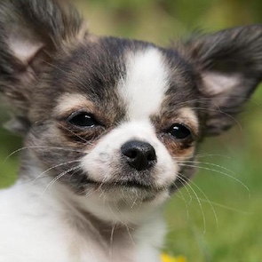
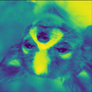
Figure 1: Dataset Preprocessing
CNN-Based Classification
Task 1 involves training a ResNet18 (RN18) (RN18VG) CNN model on the CCC dataset. The model architecture consists of 72 layers, of which, 18 are deep layers. These consist of convolutional layers, batch normalization, and residual blocks. Using the residual blocks, ResNet18 is able to bypass layers when weights begin to cause a vanishing gradient. ResNet18 has approximately 11 million trainable parameters, which are learned during the training process to optimize the network's performance on a given task. The model optimization is implemented with Stochastic Gradient Descent (SGD) using Categorical Cross-Entropy (CCE) as a loss function. This specific model (ResNet18) was chosen due to its performance capabilities and on complex datasets and its relatively low amount of learnable parameters compared to VGG 16 for example which has approximately 138 million. Essentially, the aim was to balance complexity with computation requirements, as resources are limited in the environments used. In terms of wall clock time to process the 4800 images in the training and validation sets, we averaged approximately 25 seconds per epoch with T4 GPUs.
Once the CNN model has been trained, its classification head is discarded and the encoder model, ENC1, is saved for further applications. The final step of task 1 consists on using the ENC1 on the dataset it was trained on, the CCC dataset, to extract its features. As these consist of high-dimensionality features, these are reduced with the T-Distributed Stochastic Neighbor Embedding (t-SNE) process for plot visualization.
Feature Extraction
Task 2 involves comparing features extraction from the encoder portion of the model (removal of the Fully-connected Dense layer in figure 2) of a pre-trained CNN encoder trained on ImageNet (ENC2) and the encoder developed in task 1 (ENC1) on PCC and AFC. The extracted features will undergo dimension reduction to be visualized with t-SNE. The K-nearest neighbor and Random Forest machine learning techniques will be used to classify the features extracted by ENCT1 from Dataset PCC. The Random Forest (RF) technique is chosen for its averaging/majority vote nature that reduces overfitting and enhances stability (RF1), (RF2), (RF3). A 70/30 split is used for training and testing the RF, as well as the default number of estimators (100) of the sklearn library (SKLRF). To assess the performance of all models, confusion matrices will be used to illustrate the multi-class classification and class-wise evaluation metrics (recall, accuracy and precision). The classification results from the extracted features (ENC1 on PCC) are examined for an analysis of knowledge transfer. Considering the PCC dataset and the CCC dataset (on which ENC1 was trained) share a domain, the classification results would be indicative of the effective use of transfer learning.
Results
Task 1 Results
We set up a 7:1:2 training, validation, and testing dataset split to create encoder ENC1. The validation set is used in tandem with the training set within the training loop in order to assess the hyperparameter configuration. Once the training loop has completed, we plot the training loss tracked during the training process. The test dataset portion is then used in order to verify the model's capacity for generalization. Finally, a classification report is created which displays the key metrics to evaluate the model's ability to classify such as precision, recall, etc.
We started our trials with the following hyperparameter configuration: batch size of 16, SGD with a learning rate of 0.01 and 0.9 momentum, and 15 epochs. Through experimentation, a few changes were made to facilitate convergence. Due to network instability observed in the first few epochs, the learning rate was decreased to 0.001. Fluctuations in the validation loss were detected as well, which would indicate overfitting behaviour. The batch size was increased to 32 in an attempt to mend this, which proved successful. Finally, the hyperparameters that we found more than satisfactory were the following: batch size of 32, SGD with a learning rate of 0.001 and 0.9 momentum, and 15 epochs.
The ResNet18 model trained with our hyperparameter configuration discussed previously was able to achieve CCE loss of 0.058 and the classification report in Table 2. Overall, the model performed exceptionally for all classes. Notably though, with a precision of 0.98, recall of 1.00 and F1-score of 0.99, the model was able to correctly classify the NORM images more consistently than the MUS and STR classes. This would indicate that the intricacies of the NORM images were perhaps learned marginally better.
Table 2. Task 1: Test Data Classification.
| Class | Precision | Recall | F1-score | Support |
|---|---|---|---|---|
| MUS | 0.97 | 0.96 | 0.97 | 398 |
| NORM | 0.98 | 1.00 | 0.99 | 375 |
| STR | 0.97 | 0.97 | 0.97 | 427 |
| Accuracy | 0.97 | 1200 | ||
| Macro Avg | 0.98 | 0.98 | 0.98 | 1200 |
| Weighted Avg | 0.98 | 0.98 | 0.98 | 1200 |
Once training was completed, we proceeded to remove the classification head and fed all 6000 images and applied t-SNE dimensionality reduction on the output. This was then visualized in a plot shown in Figure 1. The clear clustering indicates that the dataset classes are in fact distinguishable when their features are reduced to the 2-dimensional space.
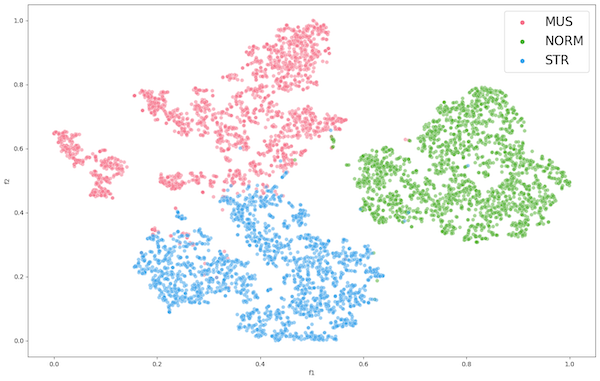
Figure 2: Encoder 1 Feature Extraction of CCC
Task 2 Results
The clustering observed in the ENC1 feature extraction of CCC (Figure 2) informs us that the model encoder can easily distinguish between the classes of the dataset using its learned features. Following the steps for task 2, we use the encoder ENC1 to extract features on datasets PCC and AFC using t-SNE for visualization.
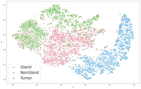
Figure 3: Encoder 1 Feature Extraction of PCC
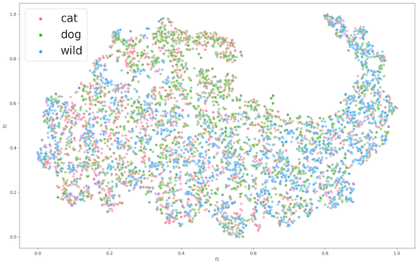
Figure 4: Encoder 1 Feature Extraction of AFC
The figure for ENC1 on the PCC dataset (Figure 2) presents the encoders mediocre separation between the gland (pink) class and the non-gland (green) class of the PCC dataset. This suggests that the learned features may not be suitable for the classification of the datasets gland and non-gland classes. Despite this, the tumor class exhibits clear distinguished features, which could be attributed to the extracted features of CCC being well aligned with tumor, rather than gland and non-gland. As for the AFC dataset (Figure 3), ENC1 failed to identify any clusters or patterns. This is to be expected because the type of images with which encoder ENC1 was trained upon are vastly different than those found in AFC, so it's the encoder would poorly classify the AFC dataset classes.
We then proceeded with the encoder ENC2 using ImageNet1K weights, extracted features from datasets PCC and AFC, and applied t-SNE as presented in Figure 4 and Figure 5 respectively. Both representations show some form of clustering, but AFC performed much better than PCC. This is to be expected because ImageNet1K was trained on over 1 million images of animals and objects. As for the PCC dataset, we can still observe decent clustering, which suggests that the pre-trained encoder learned features that had proved applicable to an extent on a dataset completely unrelated to training data.
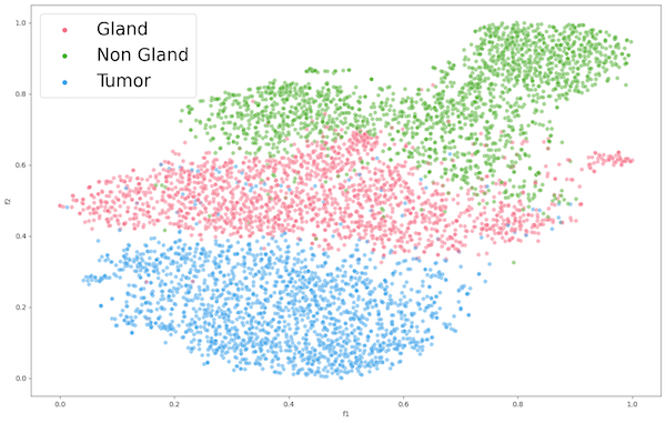
Figure 5: Encoder 2 Feature Extraction of PCC
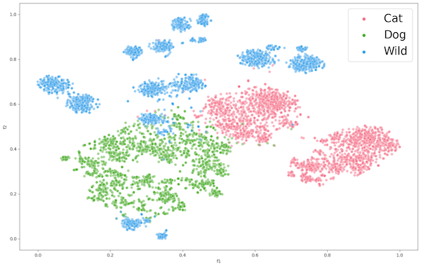
Figure 6: Encoder 2 Feature Extraction of AFC
Given the 6000 features that had been extracted previously, we then fed these features into a Random Forest classifier to discern the underlying patterns associated with our three target classes: Gland, NonGland, and Tumor. To commence, we segregated our features and labels, encoded the categorical labels numerically, and partitioned the data into training and test subsets, maintaining a 70-30 split to validate our model's predictive power on unseen data. The Random Forest number of estimators was set to 100.
Upon convergence, the model was subjected to the test set to predict the classes of the data points. The performance of the classifier was then quantified using a confusion matrix (Figure 8) and a classification report (Table 3). The classification report revealed precision, recall, and f1-scores for each class, while the confusion matrix provided a visual representation of the classifier's performance, highlighting the instances of correct and incorrect predictions.
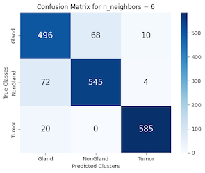
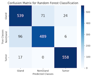
Figure 8: KNN & Random Forest Confusion Matrix PCC
Table 3: Random Forest PCC Classification.
| Class | Precision | Recall | F1-Score | Support |
|---|---|---|---|---|
| Gland | 0.83 | 0.85 | 0.84 | 634 |
| NonGland | 0.87 | 0.83 | 0.85 | 591 |
| Tumor | 0.95 | 0.97 | 0.96 | 575 |
| Accuracy | 0.88 | 1800 | ||
| Macro Avg | 0.88 | 0.88 | 0.88 | 1800 |
| Weighted Avg | 0.88 | 0.88 | 0.88 | 1800 |
The classification report reveals a well-balanced precision and recall across all categories, with the Tumor class standing out due to its high precision and recall scores. This highlights the model's capability in accurately differentiating between various classes, achieving an average accuracy rate of 88%.
Finally, we applied the k-nearest neighbors (KNN) clustering classification (SKLRNN) to our extracted feature data from PCC. The objective here was to use the supervised KNN technique to examine and classify the data. We applied KNN to the features using 6 neighbors, which through testing yielded the best results. Once finding that a KNN with 6 neighbors produced the highest accuracies, we split the data with the same 7:3 ratio, scaled the data, created our KNN classifier, trained it on our training set, and tested its performance against the test set.
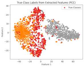
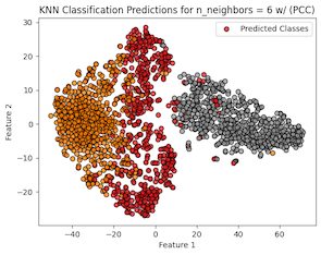
Figure 7: KNN Predictions vs True Labels PCC
Table 4: KNN PCC Classification.
| Class | Precision | Recall | F1-Score | Support |
|---|---|---|---|---|
| Gland | 0.84 | 0.86 | 0.85 | 574 |
| NonGland | 0.89 | 0.88 | 0.88 | 621 |
| Tumor | 0.98 | 0.97 | 0.97 | 605 |
| Accuracy | 0.90 | 1800 | ||
| Macro Avg | 0.90 | 0.90 | 0.90 | 1800 |
| Weighted Avg | 0.90 | 0.90 | 0.90 | 1800 |
As can be seen in Table 4, the classification report received scores of 90% for each metric, indicating a good overall performance from the KNN classifier against the extracted features. This is confirmed visually with the classification predictions from the KNN compared against the true labels (Figure 7) where for the most part (90%) the data points are correctly guessed. It is mostly in the outliers where this is not the case, which can be expected, since KNN operates on nearby data points to classify. Observing the confusion matrix in Figure 8, we see the same results, where the diagonal contains most of the data points, indicating the KNN performed well at classifying our data.